Backpropagation for Dummies

(work in progress)

Backprop is a common way to train artificial neural networks. To understand ANN it is important to understand backpropagation. The math behind it is not too hard to understand, but the intuitive reading can be somewhat confusing. This is an attempt to make it more easy to understand. I'll keep this as simple as possible, but not simpler.

Basics and terminology

We assume an ordinary neural network with the sigmoid activation function and the standard error function.

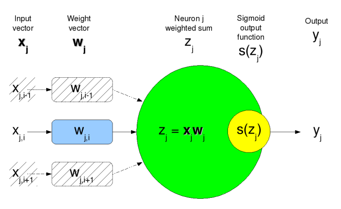
x is the input vector.
w is the weight vector.
z is the neuron weighted sum xw.
s(z) is the sigmoid output function (1+e^-z)^-1
y is the neuron output s(z)
j is the index for a particular neuron.
i is used as vector index.
E is the network total output error.

Neuron j can then be described as;

y_j = s(x_jw_j)

Graphical representation of the Neuron

An example artificial neural network

Here is a three layer network with two input units and one output unit. This toy net is able to solve problems like the logical operation Exclusive OR (xor). This operation is often used testing different training algorithms despite of the fact that the xor operation itself is not a task suitable for a neural network to solve.

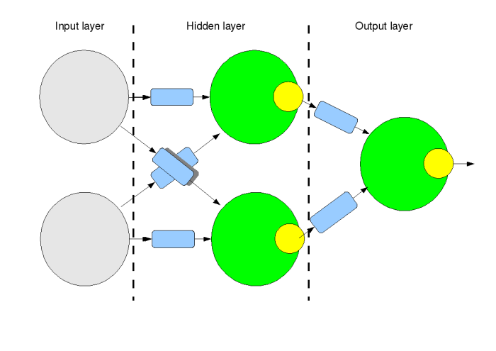
The evaluation of the network function is from left to right. The blue boxes are the weights. Assert the input values to the input layer (gray), calculate the weighted sum (green) for the following neurons and then apply the output function (yellow). Repeat for all neurons in the layer and then continue with the next layer until all neurons in all layers are done. The answer is now found on the output(s).

Please note that although this network have three layers, only two of those are actually layers of neurons. The input layer do not consists of neurons and have no weights and no output function, but only acts as an input vector to the first hidden layer.

Backward propagation

The error signal we propagate backward in the network represents how fast the network output total error changes with the weighted sum for a particular neuron z_j. Or in other words, δ is the slope (gradient) of the error surface.

δ_j = E'(z_j)

This is done recursive, and the base case is the output δ we get by the derivative of the error function with respect to the output value.

y is the network output
t is the desired target

The standard error function

E = ½(t-y)²

(sorry about multiple times, trying out some different math formula rendering add-ons)

The base case δ we seek is the derivative of the error function with respect to the output

First expand it

E(y) = ½(y² - 2ty + t²)

Derivative with respect to y

E'(y) = ½(2y - 2t) = y - t

δ_OUTPUT = E'(y) = y - t

So our base case δ is the difference of the output y and the desired target t. This is the first δ to backward propagate into the output neuron. Take a few seconds to meditate over the fact this is the derivative of the error, and not the error itself.

Here it is shown graphically for the first delta corresponding to the network output. Assume the desired target output is 0.8:

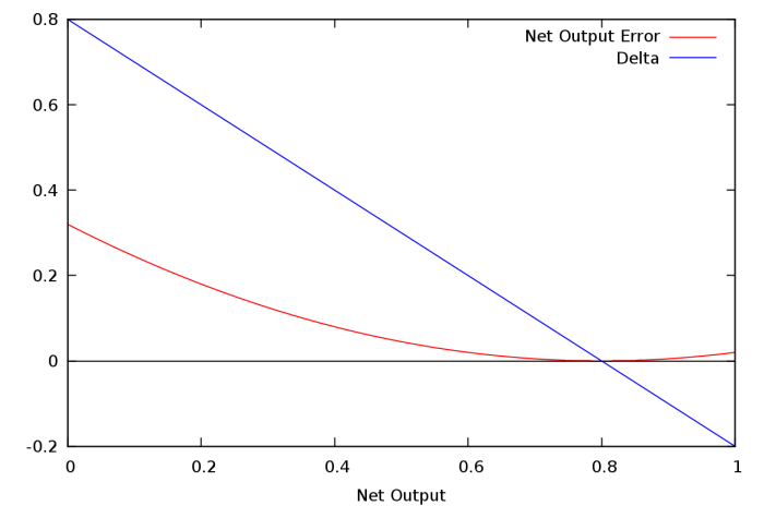
The red is the standard error function and the blue its derivative known as δ. At the solution 0.8 we see that the error is zero as well as the slope of the error function, i.e. δ.

To make it more easy to understand the similarity of this last δ and all the other, I am going to add one "dummy" at the end of the network a little like the dummy input non-neuron units. A simple one-to-one connected with a weight of 1.0 will not change the semantics of the network.

This base case δ tells us that the network total output error changes proportional with the difference of the actual and desired target output. Now we need to recursively backwards propagate this through the net. The δ we got so far corresponds to the output itself, not the output neuron. To get the δ of the output neuron we need to traverse the sigmoid output function backwards. The chain rule tells us we can multiply derivatives with each others to get the composed functions derivative.

Lets have a look at the sigmoid output function

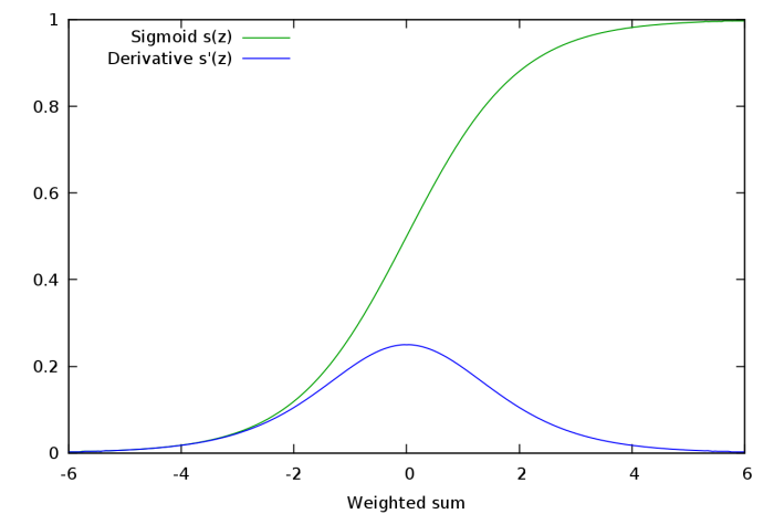
The green shows how the sigmoid function transforms the neuron weighted sum into the interval [0..1] with the steepest slope around zero. The blue derivative shows this as well. To backpropagate δ we must multiply our current δ with this derivative s'(z_j) (blue line). We know the current z_j from the forward step. It is also trivial to calculate it from y since s'(z) = y(1-y). This way we get the preceding δ. Note that the more z_j diverts from zero, the less influence this neuron get on the output error, and this independent if z_j have the desired value or not. The neurons easy get stuck at extreme values, and change very rapidly around zero. This can be seen teaching the networks; nothing happens for a long time, and then suddenly the error drops quickly.

Goals of Backprop

The goal of backprop is of course to make sure the network gives a correct result. A correct results implies that the error of the network is to be kept as low as possible. This is achieved by adjusting the weights in the network. So we formulates a part goal;

The goal is to find out how a particular weight w_j,i influences the output error of the net.

If we for each weight knows how it influences the network output error, we know how to adjust them. w_j,i is the weight to neuron j vector index i. Think of the error as a function of the weight. The derivate of this function will tell us how much a weight change effects the output error.

dE/dw_j,i is what we are seeking, or E'(w_j,i) if you prefer that notation. This is how fast the error is changing relative the weight. Especially the sign tell us in what direction the error will go if we change the weight. We often do not know very much of the curvature of the error surface, so the sign is more interesting than the value. The value of the derivative can actually be quite hazardous. If we are very far from the solution and the derivate is low, it makes us take smaller steps towards the solution than if we are closer and have a higher derivate. This small steps not only increases the time to converge, but also the risk of getting stuck in a local minimum.

We can not obtain E'(w_j,i) directly, but if we use the chain rule we see that

E'(w_j,i) = E'(z_j) * z_j'(w_j,i) (1)

So how does this help us?

The weighted sum z_j can be written as a function of the weight:

z_j(w_j) = x_j * w_j

and its derivative with respect to w_j is then of course

z_j'(w_j) = x_j

Yes, sure it feels strange to have x as a constant in the equation here, but remember it is the derivative of z_j with respect to the weight, and that the neuron input x_j is not the function input here. And see, this is what we need in equation (1) above.

The sigmoid

The sigmoid output function we need to both find its derivative and also do it from reverse. Backprop means we are going backward, so we need to fix this.

First the sigmoid derivative.

s(z) = (1+e^-z)^-1

s'(z) = s(z)(1-s(z))

And now if we assume s(z) = y as above and we get

s'(z) = y(1-y)

Can it be more simple? y(1-y) equals s'(z) from the functions output value. Make sure you realize that we calculates the derivative from the functions output value. We are going backwards. From the output of the neuron we get the value of the derivative of the output function with respect to the neurons weighted sum.

Common misconceptions

The input layer do not consists of neurons. If a neuron is defined as the picture above, the ordinary three layer network consists only of two neuron layers.

It is not the error itself that is backpropagated, but the error derivative with respect to the neuron weighted sum. This E'(z_j) describes how much the network output error is influenced by a change in the weighed sum of neuron j. This is the δ value backpropagated.

Backpropagation ... of what?!

Backprop is often referred to as backwards propagation of errors. This is at best not very descriptive. I would go as far as claim it is plain wrong. The error is the total network output error for a training input/output pattern pair.

t_p is the desired target output vector for pattern p
y_p is the actual output vector for the same pattern p.

Then the error can be described as

E = ½(t_p-y_p)²

This is the total network output error for pattern p. Why should we backpropagate this value?! No. The δ we are backward propagating is the error derivative with respect to the neuron weighted sum.

δ_j = E'(z_j)

This δ describes how much the network output error is influenced by change in the weighed sum of neuron j. You can also see this is the missing part of equation (1) above. In other words, the backward propagated δ tells us how strongly each any every neuron in the network affects the output error. An absolute high δ represents an important neuron, and a δ close to zero tells us the value of this particular neuron do not affect the output for this pattern very much at all.

We can show this mathematically. We write the error as a function of the output vector y.

E(y) = ½(t-y)²

Expand it

E(y) = ½(y² - 2ty + t²)

Derivative with respect to y

E'(y) = ½(2y - 2t) = y-t

The difference of the output and target vectors is the derivative we are seeking. This should look familiar to you if you have implemented backprop. This is used as the base case δ calculating the δ for the output units.

Again, the difference of actual output and desired output y-t is not the error, but its derivative. Claiming it is almost the error, is as claiming "speed" is almost the same as "distance". Try that the next time you get a speeding ticket. ;-)

/By Mikael Q Kuisma

Back Prop